Introduction
At Newbury last Saturday Al Ferof ran in the Denman Chase and Smad Place in the Novice Chase. Previously both horses had run below form when faced with, in Al Ferof’s case, the same 24 f Trip, and in Smad Place’s case, the same Heavy Going they faced on Saturday. In Al Ferof’s case he ran 7lb below his previous best in the 24f King George VI Chase at Kempton on Boxing Day 2013, whilst Smad Place ran 13lb below his previous best on Heavy Going in the Long Walk Hurdle at Ascot in December 2012. So how important is previous form over the same Trip, or on the same Going, in assessing prospects when the same Trip or Going is faced again? On Saturday in Al Ferof’s case he again ran below form, wheras Smad Place went on to win his race, posting his highest chase rating to date.
Data, Universe & Method
The source of the data is Raceform Interactive (RFI) with the analysis carried out in the R statistical environment. National Hunt (NH) races in the database from 2006 up to early February 2014 are considered. Each time a horse runs its Racing Post Rating (RPR) is compared with the maximum RPR the horse has achieved up to and including race date. The difference between the two numbers is defined as the RPR relative (RPRrel). The maximum value RPR can achieve is zero. Following Timeform’s definition, if a horse runs within 5lb of its maximum rating it is considered to have Run To Form (RTF) – horses are then classified into two categories – either having RTF (given a 1) or below (given a 0). The Going on which races took place were classified into four categories: Quick, Good, Soft and Heavy. The distance over which races were run were classified into five Trip categories of: up to 17f, between 17f and 21f, between 21f and 25f, between 25f and 29f, and 29f plus.
To assess the importance of previous form given the Going or Trip, the RTF classification as at a particular race (1 or 0 ) is then compared with the RTF classification achieved (1 or 0) in its next race. All of the previous races at the Going or Trip are used to determine the classification, so if a horse has RTF on any occasion in the past it is allocated a 1. Horses that haven’t run on the Going or over the Trip are excluded.
In the jargon the result is a 2×2 contingency table for each Going and Trip category that can be assessed for statistical significance using a chi-squared statistic.
Going Analysis
Each of the 2×2 contingency tables for the four Going categories is presented in Table 1 below, with the number of observations given in parentheses. Classification by previous RTF is given in the first column, by subsequent performance in the second and third columns. Horses that have RTF in the past have about a one in three chance of repeating, for horses that haven’t RTF the chances are just over one in four. The results are highly statistically significant.
| Quick (29,127) | Below | RTF | Good (134,422) | Below | RTF | |
| Below | 74% | 26% | Below | 72% | 28% | |
| RTF | 65% | 35% | RTF | 68% | 32% |
| Soft (46,127) | Below | RTF | Heavy (32,971) | Below | RTF | |
| Below | 74% | 26% | Below | 75% | 25% | |
| RTF | 68% | 32% | RTF | 68% | 32% |
Table 1: 2×2 Contingency Tables (RTF vs. Below Form) for Going Categories
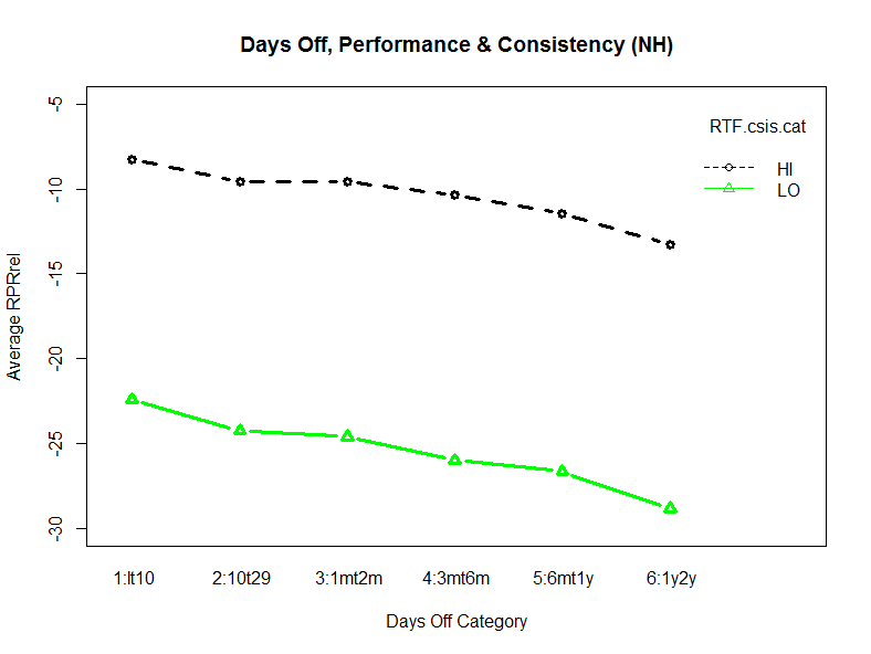
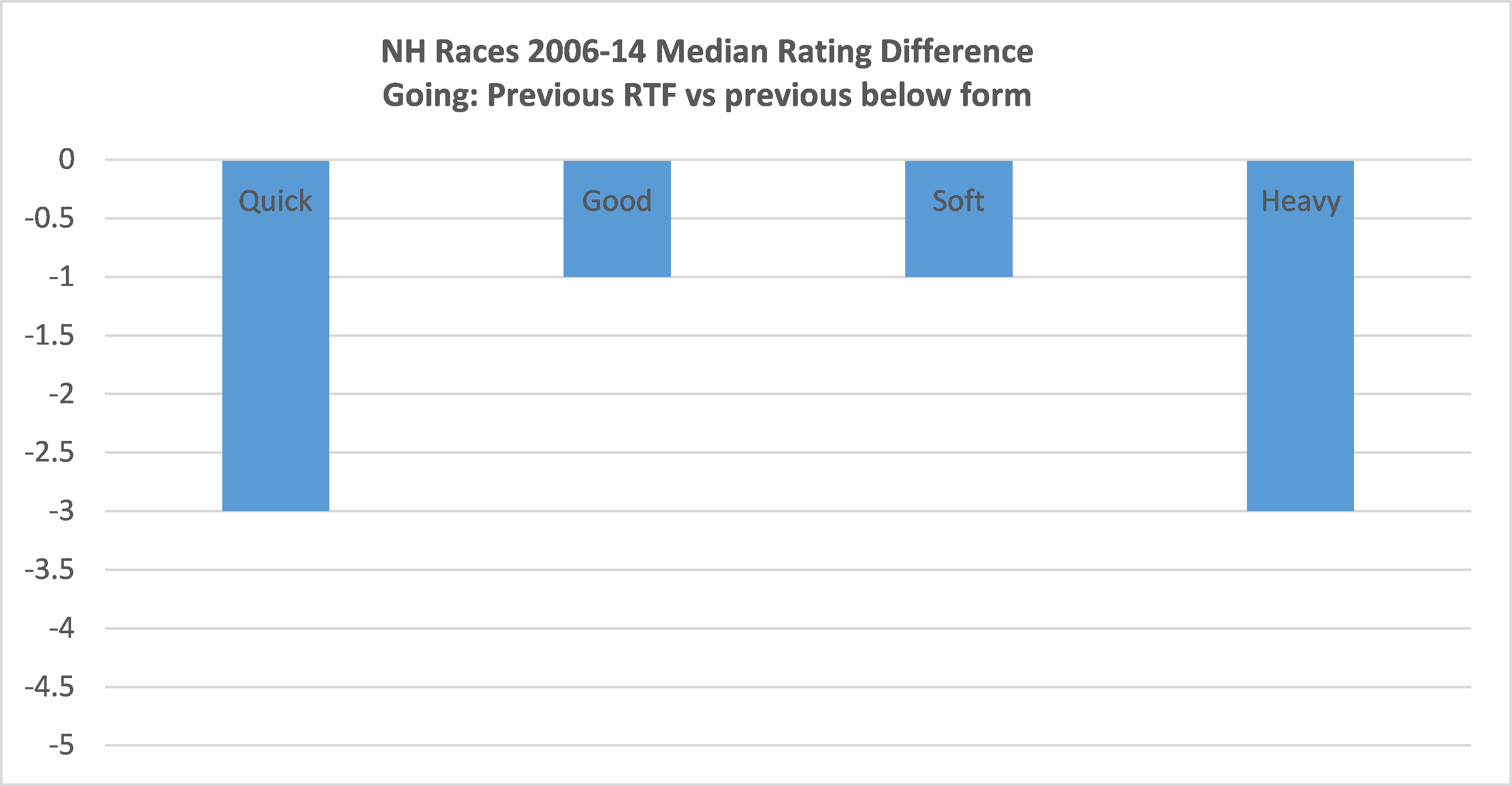
The extent of the difference in performance can be see in the graph below, which shows median differences for the four Going categories. Extremes of Going exhibit greater differences, with a range of between 1 and 3lbs.
Trip Analysis
Each of the 2×2 contingency tables for the five Trip categories is presented in Table 2 below, with the number of observations given in parentheses. Classification by previous RTF is given in the first column, by subsequent performance in the second and third columns. Horses that have RTF in the past have a decreasing chance of delivering a RTF performance next time out as Trip distance increases. This is probably because horses become more exposed as they are stepped up in Trip. In all cases, however, horses that have previously RTF outperform those that have not. The results are again highly statistically significant.
| up to 17f (86,133) | Below | RTF | 17f – 21f (91,666) | Below | RTF | |
| Below | 66% | 34% | Below | 74% | 26% | |
| RTF | 61% | 39% | RTF | 68% | 32% |
| 21f – 25f (65,248) | Below | RTF | 25f – 29f (9,036) | Below | RTF | |
| Below | 78% | 22% | Below | 80% | 20% | |
| RTF | 71% | 29% | RTF | 75% | 25% |
| 29f plus (1,565) | Below | RTF | ||||
| Below | 85% | 15% | ||||
| RTF | 79% | 21% |
Table2: 2×2 Contingency Tables (RTF vs. Below Form) for Trip Categories
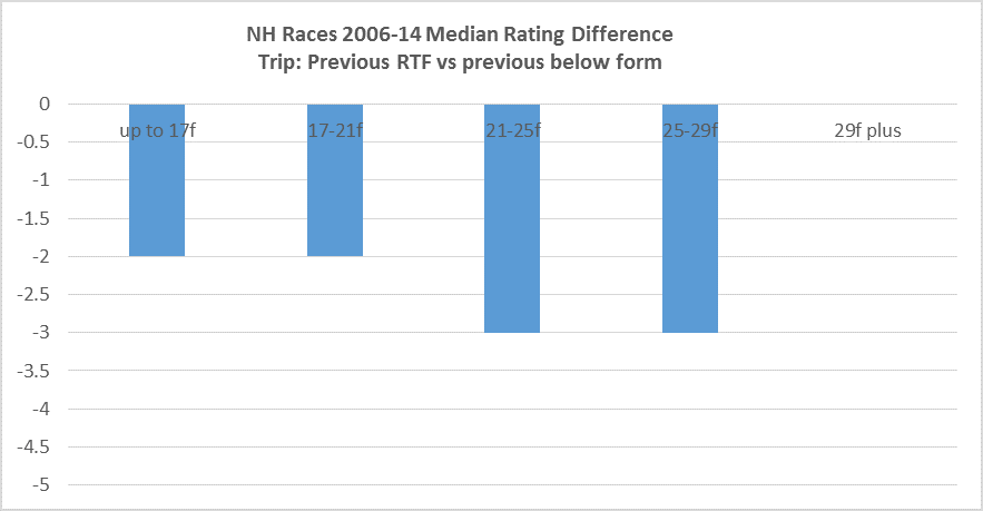
The extent of the difference in performance can be see in the graph below, which shows median differences for the five Trip categories. Differences are greatest when horses race between 21f – 29f. There is no difference in medians at 29f plus, however there is a difference in means.
Summary
If a horse has previously RTF over a particular type of Going or Trip in NH races, it is significantly more likely to do so than horses that have not. Differences in probabilities are between 5-7%, ratios substantially higher. The difference in median performance ranges between 0 and 3lbs. One possible confounding influence is the effect of horses that run consistently to form regardless of Going or Trip. However if this were the overriding effect it might be expected that the difference in performance seen in the graphs would be constant across Going and Trip categories. This is not the case. Analysis using ANOVA (analysis of variance) would answer this concern more fully.